Windows INDX Slack Parser (wisp)

Introduction

wisp is a prototype version of a Windows parser that targets NTFS index type attributes. The NTFS index attribute points to one or more INDX records. These records contain index entries that are used to account for each item in a directory. An index item represents either a file or a subdirectory and includes enough metadata to contain the name, modified/access/MFT changed/birth (MACB) timestamps, size (if it is a file vice subdirectory), as well as MFT entry numbers of the item and its parent. The wisp tool, in its simplest form, is able to walk these structures, read the metadata, and report which index entries are present.

As a directory's contents are changed, the number of valid index entries grows or shrinks, as appropriate. As more directory entries are added, eventually it will exceed the existing INDX record allocation space. At this point the operating system will allocate an additional INDX record in the size of 0x1000 byte chunk. Conversely, when entries are removed from the directory, the INDX record space is not necessarily deallocated. Thus, anytime the number of index entries shrinks, the invalid ones potentially can be harvested from the slack space. The slack space is defined to be the allocated but unused space. By comparing both the valid entries and those still in the slack space, one can make some inferences about whether a file (or subdirectory) was present in the past.

A good tutorial on harvesting index entries from INDX slack space can be found on Willi Ballenthin's webpage [4] and his DFIRonline presentation [5].

wisp uses the NTFS and index attribute parsing engine that is used in the ntfswalk tool [6] available from the TZWorks LLC website. Currently there are compiled versions for Windows, Linux and Mac OS-X.

INDX Attributes (Format/Internals)

NTFS uses two types of index attributes to store directory items: (a) INDEX_ROOT and the (b) INDEX_ALLOCATION. The former is meant for is a small number of index items, since it is resident within the file record of the MFT entry. The term resident means the data is stored within the file record's space, which is limited to a fixed size. Since the file record needs this fixed space to store its other attributes as well, there is only enough space to store only a few index entries, which are reserved for the root directory indexes. These leads to the latter attribute which is classified as non-resident. The non-resident quality of the INDEX_ALLOCATION attribute allows any associated data to exist as one or more separate 'cluster runs' within the NTFS volume. Consequently, the data associated with this attribute can grow to whatever size is needed to account for all the index items identified in a directory. There is a good explanation of these two specific attributes in Brian Carrier's book on File System Forensic Analysis [3] as well as other sources online [1, 2]. While wisp parses both attributes identified above, it is the latter attribute that contains sufficient slack space for wisp to analyze older index entries.

When parsing index attributes (or any NTFS attribute for that matter), is useful to take each attribute apart at the most basic level and extract all the fields to find the best way to analyze it. For example, when looking at any directory on the file system that contains more than a few index entries, one should be able to see both the INDEX_ROOT and INDEX_ALLOCATION attributes. Below is a snapshot of the attributes of interest for the some arbitrary directory. For clarity, all the attributes have been trimmed out with the exception of the INDEX_ROOT and INDEX_ALLOCATION attributes, since this is what wisp will analyze. One can see that the INDEX_ROOT entry which is resident only has 176 (0xb0) bytes allocated for data, while the INDEX_ALLOCATION attribute has 12288 (0x3000) bytes allocated for data. Both attributes must be parsed to give one a complete picture of all the index entries associated within a directory. Therefore, wisp will first pull out the data from the resident attribute and parse it. Next, it will identify the cluster run(s) for the non-resident data, read the clusters, fix-up the INDX records, and extract each index entry found.

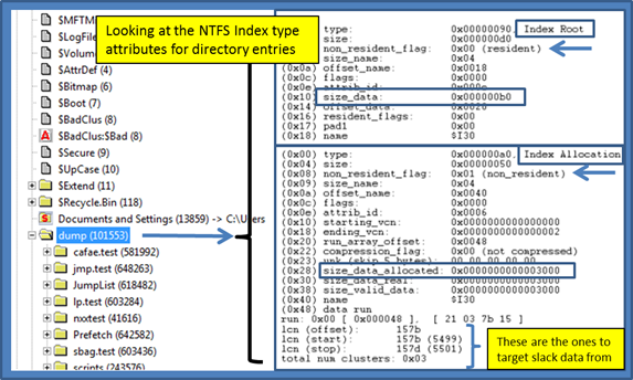
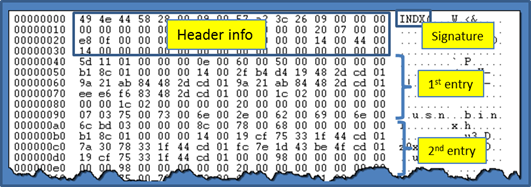
Upon examining non-resident INDX records, one can immediately see each INDEX_ALLOCATION record starts with the signature 'INDX' followed by some metadata. Some of the metadata allows one to verify the integrity of the INDX record as well as fix-up the record on sector boundaries. Also included in the header info is a DIRECTORY_INDEX record to identify the space used to store all the index entries. For details on the structure makeup, see ref [1, 2, or 3]. After the header information, the index entries follow. These are parsed by wisp to enumerate both valid index entries and those which are in slack space.

How to use wisp

While the wisp tool doesn't require one to run with administrator privileges, without doing so will restrict one to only looking at off-line 'dd' images. Therefore to perform live processing of volumes, one needs to launch the command prompt with administrator privileges.

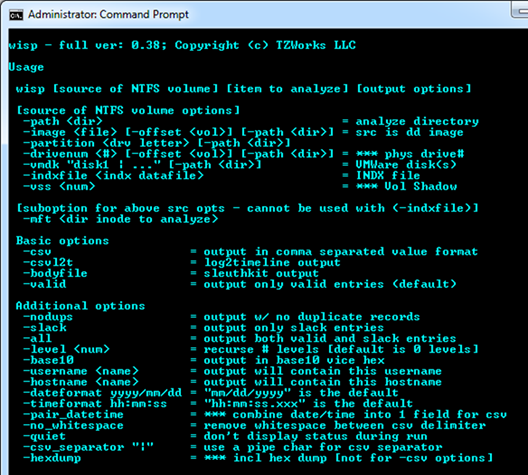
One can display the menu options by typing in the executable name with no parameters. A screen shot of the menu is shown below. From the available options, one can process NTFS INDX records with a handful of 'use-cases'. Specifically, wisp allows processing from any of these sources: (a) live volume, (b) 'dd' type image, (c) VMWare volume or (d) separately extracted INDX type record.

After selecting the source of the data, one can either: (a) process a single directory on the file system, (b) recursively process the subdirectories to some specified level, or (c) process all the index entries in an entire volume. Processing every directory in the entire volume is not explicitly shown in the above menu since it is the default option.

If one only wants a certain type of index entry, one can select: (a) just show valid index entries, (b) just show index entries in the slack space, or (c) both. For default output, the data is represented as unstructured text. If parsable output is desired (or something that can be displayed in a spreadsheet application), one can select from 3 options that allow for structured output (CSV, log2timeline CSV, or SleuthKit body-file). The other useful option is the 'no duplicates' choice to minimize any redundancy in the output. There is a discussion of why one might want to use the 'no duplicates' option in a later section.

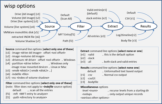
Since there are a number of possible combinations of options, the figure below shows the possible choices and where they apply in a logical processing flow. The comments in the figure annotate any restrictions for a particular option.

Parsing a Live Volume

To parse INDX entries from a live NTFS volume (or partition), one has two choices: (a) specify the volume directly by using the –partition <drive letter> option or (b) specify the drive number and volume offset by using the –drivenum <num> –offset <volume offset> option. Either choice accomplishes the same task. The first choice is more straightforward and easier to use. The second choice, while more complex, allows one to target hidden NTFS partitions that do not have a drive letter.

The next step is to decide what you want to target. The choices are: (a) a specific directory on the file system (specified by either the –mft or –path options), (b) a collection of subdirectories within a directory (how deep you wish to go is specified by the –level option) or (c) all directories (specified by the –scanall option). A couple examples are shown below:

    wisp –partition c –path c:\$Recycle.Bin –level 2 –all –csv > results1.csv
    wisp –drivenum 0 –offset 0x100000 –all –csv > results2.csv

The first example targets the hidden directory of c:\$Recycle.Bin, and the –level 2 switch tells wisp to include any subdirectory in the analysis, up to 2 levels deep. The –all switch means both valid and invalid (slack) entries will be included in the output. Finally, the output is redirected to a file and the format is CSV.

The second example uses the same output options as the first, but now targets the first physical hard drive. The hex value 0x100000 is specified as the offset to the volume (or partition) we wish to analyze. For this example, this happens to be the hidden partition created during a Windows 7 installation. Since there is no –mft or –path options explicitly listed, the implication to wisp is we want to traverse the entire volume parsing all INDX records associated with the volume.

Parsing an Image File off-line

To process an image that has been already acquired and is in the 'dd' format, one uses the –image switch. This option can be used in two flavors. If the image is of an entire drive then one needs to explicitly specify the offset of the location of the volume you wish to target. On the other hand, if the image is only of a volume, then you do not need to specify the offset of the volume (since it is presumed to be at offset 0).

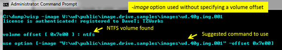
For the first case, where an offset needs to be explicitly specified, wisp will help the user in locating where the NTFS volume offsets are. If one just issues the –image command without the offset, and there is not a NTFS volume at offset 0 (eg. second case mentioned above), wisp will proceed to look at the master boot record contained in the image, determine where the NTFS partitions are, and report them to the user. This behavior was meant to be an aid to the user so that one does not need to resort to other tools to determine where the offsets for the NTFS volumes are in an image. Below is a screenshot what is displayed to the user in this situation.

Shown in the screenshot is a –image command that is issued without the offset. wisp detects that the image is of an entire drive vice of a volume and locates one NTFS volume at offset 0x7e00 hex. wisp then reports to the user a suggested syntax (of the command, if re-issued) to process this volume.

Another nuance with using images as the source, is when specifying a path to a directory within the image to analyze, using the –path option. Since the image is not mounted as a drive, one really should not associate it with a drive letter when specifying the path. If one does do this, wisp will ignore the drive letter and proceed to try to find the path starting at the root directory which is at MFT entry 5 for NTFS volumes.

Below are two examples of processing 'dd' type images: (a) the first analyzes an entire volume at drive offset 0x100000 hex and (b) the second analyzes an image of a volume starting at the path "Users".

    wisp –image c:\dump\my_image.dd –offset 0x100000 –all –csv > results1.csv
    wisp –image c:\dump\vol_image.dd –path "\Users" –level 5 –all –csv > results2.csv

While the first example traverses the entire volume, the second starts at the "Users" directory and recursively processes the subdirectories up to 5 levels deep. Notice the second example does not specify an offset, since the image is of a volume (meaning the volume starts at offset 0) while the first is an image of a drive and the first NTFS volume starts at offset 0x100000 hex.

Both examples extract valid and invalid index entries as well as redirect their output to a file using CSV formatting.

Parsing a NTFS Volume Mounted on Linux or Mac OS-X

Sometimes you do not have a 'dd' image of a volume or drive, but instead have the physical hard drive available you wish to analyze. If you are running wisp in Windows, then one can mount the physical dirve and proceed to follow the guidelines in the earlier section for parsing a live volume. However, if you are running wisp in Linux or Mac OS-X, you should also be able to mount the target drive as well. Once it is successfully mounted, one uses the –image <device name of drive or volume> –offset <offset to desired volume, if a drive> option to access the appropriate NTFS volume. Below is an example of how to do this using a Mac box.

Assuming one has the proper setup with write blocker and hard drive shuttle, after connecting the Windows drive to the Mac, one can issue the diskutil list command to enumerate all the drives and volumes mounted on the machine. For our configuration under test, the results showed the following:

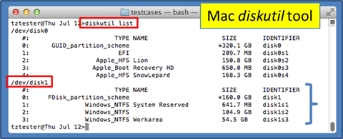
The second disk (designated as /dev/disk1) is the external disk that was plugged in, and it consisted of 3 NTFS partitions (disk1s1, disk1s2, disk1s3). Once the device for the disk has been identified, one can reference the partitions directly with their respective identifiers. If for some reason, the diskutil does not identify the partitions due to disk corruption, one can also reference the disk directly and explicitly give the offset of the desired partition one wishes to operate on. Below is how one could use wisp to help identify the partition offsets.

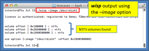
Notice, the command that was issued above was just the device name of the disk and wisp looked at the MBR to determine where the NTFS partitions were located relative to the start of the disk. Also notice the notation of /dev/rdisk# is used. The 'r' is (which is unique to Mac) used to specify we want to access the drive as raw I/O as opposed to buffered I/O. The buffering is nice for normal reads/writes, but it is much slower when traversing in chunks aligned on sector boundaries.

Based on the above discussion, below are the possible options to access the first NTFS volume.

    sudo wisp –image /dev/rdisk1s1 –all –csv –nodups > out.csv
    sudo wisp –image /dev/rdisk1 –offset 0x100000 –all –csv –nodups > out.csv

Notice the 'sudo' in front of the wisp command. This will allow wisp to run with administrative privileges to access the raw drive.

Linux is similar to Mac, but instead of using the diskutil tool, one would use the df tool to enumerate the mounted devices.

Parsing a VMWare Volume

Occasionally it is useful to analyze a VMWare image containing a Windows volume, both from a forensics standpoint as well as from a testing standpoint. This option is still considered experimental since it has only been tested on a handful of configurations. Furthermore, this option is limited to monolithic type VMWare images versus split images. In VMWare, the term split image means the volume is separated into multiple files, while the term monolithic virtual disk is defined to be a virtual disk where everything is kept in one file. There may be more than one VMDK file in a monolithic architecture, where each monolithic VMDK file would represent a separate snapshot. More information about the monolithic virtual disk architecture can be obtained from the VMWare website [10].

When working with virtual machines, the capability to handle snapshot images is important. Thus, if processing a VMWare snapshot, one needs to include the snapshot/image as well as its inheritance chain.

wisp can handle multiple VMDK files to accommodate a snapshot and its descendants, by separating multiple filenames with a pipe delimiter and enclosing the expression in double quotes. In this case, each filename represents a segment in the inheritance chain of VMDK files (eg. –vmdk "<VMWare NTFS virtual disk-1> | .. | <VMWare NTFS virtual disk-x>" ). To aid the user in figuring out exactly the chain of descendant images, wisp can take any VMDK file (presumably the VMDK of the snapshot one wishes to analyze) and determine what the descendant chain is. Finally, wisp will suggest a chain to use.

Aside from the VMDK inheritance chain, everything else is the same when using this option to that of normal 'dd' type images discussed in the previous section.

Two Categories of Slack entries

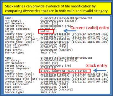
The slack entries in the output have comments associated with them. The comments come in 2 categories: (a) entries that have not been deleted and (b) those that have been deleted. These categories are best shown with an example. Using the default output option, 2 snapshots are shown below.

The first snapshot shows a valid index entry as well as an invalid index entry. Both index entries point to the same file (one can tell this since the MFT entry number and sequence numbers match up). The difference, aside from the fact one is in slack space, is some of the MACB timestamps are different as well as the size of the file. wisp annotates the modification with a comment, denoted by [m.c.] and [size] in the snapshot below. The [m.c.] translates to the modify timestamp and 'MFT change' timestamps, respectively, as being different than the valid entry. The [size] notation just means the size of the file has changed. From this, one can get some past data on a file that has gone through some revisions.

For the second case, shown in the below snapshot, wisp just annotates the slack entry as deleted. The term deleted here is only accurate in the sense that this index entry is no longer part of the directory containing the INDX record(s). Whether the item was moved to another subdirectory or actually deleted is unknown from the data presented here.

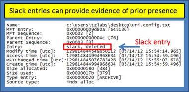
Finally, looking at the data available in an index entry one can see the MACB timestamps and size, as well as the MFT entry metadata, flags and source of information. The MACB timestamps should match the standard information MACB timestamps of the file/subdirectory.

Extracting Clusters Associated from a Deleted Entry

At this point in the analysis, one may want to go deeper and try to find if the deleted file is still available by trying to find the 'cluster run' data associate with the MFT entry. Since the INDX records do not have any cluster run data associated with an index entry, one would need to use the MFT entry specified and then use some other tool to read the file record associated with that MFT entry. One could extract the data either from the local volume or from the volume shadow copy store. If pulling from the local volume, one can use the ntfscopy utility [7] from TZWorks. This tool will allow one to (a) input a volume (live or off-line), (b) specify the desired MFT entry to copy from and (c) output the extract the data associated with the MFT's cluster run as well as the metadata associated with that MFT entry. Below is an example of doing this with ntfscopy using the MFT entry number 645130, which is for the slack entry shown above.

    ntfscopy –mft 645130 –dst c:\dump\645130.bin –partition c: –meta

For details on the ntfscopy syntax, refer to the ntfscopy readme file [7]. Briefly, the –mft option allows one to specify a source MFT entry to copy from. The –meta option says to create a separate file (in addition to the copied file) that contains the metadata information about the specified MFT entry. The metadata file will be created with the same name as the destination file with the appended suffix .meta.txt. Included in the metadata file are many of the NTFS attributes of the target source file (or MFT entry). This includes, amongst other things, the cluster run and MACB timestamps. From the metadata one can see if the MFT sequence number is the same or not (which would be the indication whether the MFT record was assigned to another file or not).

Eliminating the Duplicates

For those INDX records that have many slack entries, it is not uncommon for there to be quite a few duplicate entries that are parsed and displayed in the output. Duplicate here means the filename and MACB timestamps are the same, however the location of the entry in the INDX record is different. For every unique location in the INDX record, wisp will happily parse the index entry and report its findings to the investigator. This can be quite annoying when some entries have more than a few duplicates and one is trying to wade through a lot of data; especially when carving out entries from slack data on all the directories in an entire volume.

To get rid of duplicates, one can invoke the –nodups switch. This tells wisp to analyze the data extracted and only report one instance of the entry. One thing to be aware of when using this option, is that wisp will internally always analyze valid and slack entries independent of what the user selects as input options. After all the data is extracted, wisp will start deciding if there are duplicate entries or not. It does this by looking at comparing all slack entries with valid entries to see if there is a duplicate, and if not, they are compared to any slack entries that have been marked as non-dups. What this means is, if one runs wisp and only wants non-duplicate slack entries, some slack entries will not be reported if there are valid entries present that are the same.

For more information

The user's guide can be viewed here

If you would like more information about wisp, contact us via email.

Downloads

		Intel 32-bit Version	Intel 64-bit Version	ARM 64-bit Version
	Windows:	wisp32.v.0.58.win.zip	wisp64.v.0.58.win.zip	wisp64a.v.0.58.win.zip		md5/sha1
	Linux:	wisp32.v.0.58.lin.tar.gz	wisp64.v.0.58.lin.tar.gz	wisp64a.v.0.58.lin.tar.gz		md5/sha1
	Mac OS X:	Not Available	wisp.v.0.58.dmg	wisp.v.0.58.dmg		md5/sha1
		*32bit apps can run in a 64bit linux distribution if "ia32-libs" (and dependencies) are present.